This time I will show you how to build a simple “AI” product with transfer learning. We will build a “dog breed identification chat bot”. In this first post, I will show how to build a good model using keras, augmentation, pre-trained models for transfer learning and fine-tuning. In the following posts I will first show you how to build the bot app with telegram and then how to deploy the app on AWS.
We will use the dataset from kaggle, which is a subset of ImageNet that only contains images of dogs. This post is structured as follows:
- First we load and inspect the data.
- Then we select a pretrained model, the xception model because it's memory footprint is comparable small (88Mb, since we want to deploy it on AWS we are interested in a small size)
- Then we add more layers on top of the pretrained model and use data augmentation to improve the performance
- Now we explore the power of cyclical learning rates
- In the end we fine-tune some of the convolutional layers of the pretrained network, to boost the performance even further.
import numpy as np
import pandas as pd
import matplotlib.pyplot as plt
from mpl_toolkits.axes_grid1 import ImageGrid
from os import listdir, makedirs
from os.path import join, exists, expanduser
from tqdm import tqdm
from sklearn.metrics import log_loss, accuracy_score
Look at the dataset
We will have 120 different dog breeds we want to identify.
NUM_CLASSES = 120
SEED = 2018
data_dir = 'data/'
labels = pd.read_csv(join(data_dir, 'labels.csv'))
sample_submission = pd.read_csv(join(data_dir, 'sample_submission.csv'))
print("Number of samples: {}".format(len(listdir(join(data_dir, 'train')))))
Number of samples: 10222
(labels
 .groupby("breed")
 .count()
 .sort_values("id", ascending=False)
 .head(10)
)
| id | |
|---|---|
| breed | |
| scottish_deerhound | 126 |
| maltese_dog | 117 |
| afghan_hound | 116 |
| entlebucher | 115 |
| bernese_mountain_dog | 114 |
| shih-tzu | 112 |
| great_pyrenees | 111 |
| pomeranian | 111 |
| basenji | 110 |
| samoyed | 109 |
So scottish_deerhound is the most common breed…
(labels
 .groupby("breed")
 .count()
 .sort_values("id", ascending=False)
 .tail(10)
)
| id | |
|---|---|
| breed | |
| tibetan_mastiff | 69 |
| german_shepherd | 69 |
| giant_schnauzer | 69 |
| walker_hound | 69 |
| otterhound | 69 |
| golden_retriever | 67 |
| brabancon_griffon | 67 |
| komondor | 67 |
| briard | 66 |
| eskimo_dog | 66 |
and eskimo_dog the least common.
Now we split the dataset in a train and a validation set.
from sklearn.preprocessing import LabelEncoder
label_enc = LabelEncoder()
np.random.seed(seed=SEED)
rnd = np.random.random(len(labels))
train_idx = rnd < 0.9
valid_idx = rnd >= 0.9
y_train = label_enc.fit_transform(labels["breed"].values)
ytr = y_train[train_idx]
yv = y_train[valid_idx]
Next we look at some sample images and their labels.
from keras.preprocessing import image
from keras.applications import xception

def read_img(img_id, train_or_test, size):
    """Read and resize image.
    # Arguments
        img_id: string
        train_or_test: string 'train' or 'test'.
        size: resize the original image.
    # Returns
        Image as numpy array.
    """
    img = image.load_img(join(data_dir, train_or_test, '{}.jpg'.format(img_id)), target_size=size)
    return image.img_to_array(img)
Using TensorFlow backend.
import matplotlib.pyplot as plt
%matplotlib inline

def show_img(img, label, ax):
    ax.imshow(img / 255.)
    ax.text(10, 200, 'LABEL: {}'.format(label), color='k', backgroundcolor='w', alpha=0.8)
    ax.axis('off')


fig = plt.figure(1, figsize=(16, 16))
grid = ImageGrid(fig, 111, nrows_ncols=(3, 3), axes_pad=0.05)
for i, idx in enumerate(np.random.choice(list(range(10000)), size=9)):
    ax = grid[i]
    show_img(read_img(labels['id'][idx], "train", (299, 299)), label=labels['breed'][idx], ax=ax)
plt.show()
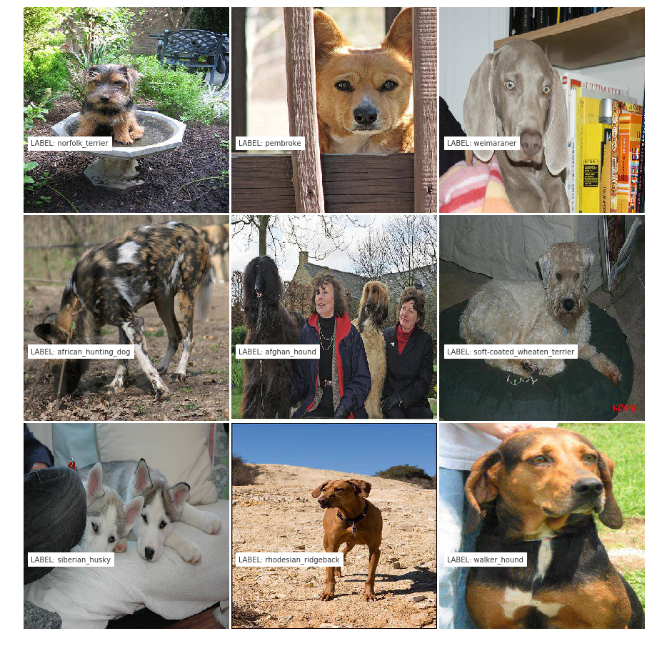
Well, it looks like dogs. So far, so good. Now we set up the first model and see how we can do.
Load the data
# options
INPUT_SIZE = 299
BATCH_SIZE = 16
x_train = np.zeros((train_idx.sum(), INPUT_SIZE, INPUT_SIZE, 3), dtype='float32')
x_valid = np.zeros((valid_idx.sum(), INPUT_SIZE, INPUT_SIZE, 3), dtype='float32')
train_i = 0
valid_i = 0
for i, img_id in tqdm(enumerate(labels['id'])):
    img = read_img(img_id, 'train', (INPUT_SIZE, INPUT_SIZE))
    x = xception.preprocess_input(np.expand_dims(img.copy(), axis=0))
    if train_idx[i]:
        x_train[train_i] = x
        train_i += 1
    elif valid_idx[i]:
        x_valid[valid_i] = x
        valid_i += 1
print('Train Images shape: {} size: {:,}'.format(x_train.shape, x_train.size))
10222it [00:29, 350.92it/s]
Train Images shape: (9174, 299, 299, 3) size: 2,460,494,322
First we set up a simple image generator for data augmentation. This means we randomly apply one or multiple transformations to an image. For example we zoom in or out for maximal 25% or we flip the image horizontally.
from keras.preprocessing.image import ImageDataGenerator

train_datagen = ImageDataGenerator(rotation_range=45,
                                   width_shift_range=0.2,
                                   height_shift_range=0.2,
                                   shear_range=0.2,
                                   zoom_range=0.25,
                                   horizontal_flip=True,
                                   fill_mode='nearest')

test_datagen = ImageDataGenerator()
Cyclical Learning rates
Another neat trick is the use of cyclical learning rates. A cyclical learning rate is a policy of learning rate adjustment that increases the learning rate off a base value in a cyclical nature. We also lower the maximum learning rate over time with a exponential decay following these formulas
cycle = np.floor(1+iterations/(2*step_size))
x = np.abs(iterations/step_size - 2*cycle + 1)
lr = base_lr + (max_lr-base_lr)*np.maximum(0, (1-x))
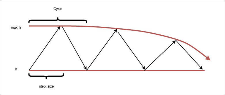
One reason this approach may work well is because increasing the learning rate is an effective way of escaping saddle points. By cycling the learning rate, we’re guaranteeing that such an increase will take place if we end up in a saddle point. The code for the keras callback can be found here and more details can be found in Leslie Smith’s paper “Cyclical Learning Rates for Training Neural Networks” arXiv:1506.01186v4.
Fine-tune Xception
Set up the model
from keras.layers import GlobalAveragePooling2D, Dense, BatchNormalization, Dropout
from keras.optimizers import Adam, SGD, RMSprop
from keras.models import Model, Input
Keras includes a lot of pretrained models. We select the Xception model because it offers a good performance with comparable small size. On top of the pretrained model we add a fully connected layer with $1024$ neurons and some Dropout.
# create the base pre-trained model
base_model = xception.Xception(weights='imagenet', include_top=False)

# add a global spatial average pooling layer
x = base_model.output
x = BatchNormalization()(x)
x = GlobalAveragePooling2D()(x)
# let's add a fully-connected layer
x = Dropout(0.5)(x)
x = Dense(1024, activation='relu')(x)
x = Dropout(0.5)(x)
# and a logistic layer -- let's say we have NUM_CLASSES classes
predictions = Dense(NUM_CLASSES, activation='softmax')(x)

# this is the model we will train
model = Model(inputs=base_model.input, outputs=predictions)
Prepare for fine-tuning
import datetime
from keras.callbacks import EarlyStopping, ModelCheckpoint, CyclicLR

# checkpoints
early_stopping = EarlyStopping(monitor='val_acc', patience=5)
STAMP = "{}_dog_breed_model".format(datetime.date.today().strftime("%Y-%m-%d"))

bst_model_path = "models/{}.h5".format(STAMP)
model_checkpoint = ModelCheckpoint(bst_model_path,
                                   save_best_only=True,
                                   save_weights_only=True)

# Authors suggest setting step_size = (2-8) x (training iterations in epoch)
step_size = 2000
clr = CyclicLR(base_lr=0.0001,
               max_lr=0.001,
               step_size=step_size,
               mode='exp_range',
               gamma=0.99994)
# first: train only the top layers (which were randomly initialized)
# i.e. freeze all convolutional Xception layers
for layer in base_model.layers:
    layer.trainable = False

# compile the model (should be done *after* setting layers to non-trainable)
optimizer = RMSprop(lr=0.001, rho=0.9)
model.compile(optimizer=optimizer,
              loss='sparse_categorical_crossentropy',
              metrics=["accuracy"])
Train the model
# train the model on the new data for a few epochs
hist = model.fit_generator(train_datagen.flow(x_train, ytr, batch_size=BATCH_SIZE),
                           steps_per_epoch=train_idx.sum() // BATCH_SIZE,
                           epochs=50, callbacks=[early_stopping, model_checkpoint, clr],
                           validation_data=test_datagen.flow(x_valid, yv, batch_size=BATCH_SIZE),
                           validation_steps=valid_idx.sum() // BATCH_SIZE)
Epoch 1/50
573/573 [==============================] - 97s 170ms/step - loss: 2.7320 - acc: 0.3932 - val_loss: 0.4863 - val_acc: 0.8577
Epoch 2/50
573/573 [==============================] - 95s 165ms/step - loss: 1.2324 - acc: 0.6626 - val_loss: 0.4245 - val_acc: 0.8595
Epoch 3/50
573/573 [==============================] - 95s 165ms/step - loss: 1.2646 - acc: 0.6848 - val_loss: 0.4257 - val_acc: 0.8614
Epoch 4/50
573/573 [==============================] - 94s 165ms/step - loss: 1.3367 - acc: 0.6894 - val_loss: 0.4582 - val_acc: 0.8498
Epoch 5/50
573/573 [==============================] - 95s 165ms/step - loss: 1.2192 - acc: 0.7064 - val_loss: 0.4185 - val_acc: 0.8663
Epoch 6/50
573/573 [==============================] - 94s 165ms/step - loss: 1.1309 - acc: 0.7192 - val_loss: 0.4344 - val_acc: 0.8643
Epoch 7/50
573/573 [==============================] - 95s 165ms/step - loss: 1.0400 - acc: 0.7356 - val_loss: 0.3920 - val_acc: 0.8798
Epoch 8/50
573/573 [==============================] - 94s 164ms/step - loss: 1.0034 - acc: 0.7397 - val_loss: 0.4005 - val_acc: 0.8702
Epoch 9/50
573/573 [==============================] - 94s 165ms/step - loss: 1.0000 - acc: 0.7389 - val_loss: 0.4180 - val_acc: 0.8624
Epoch 10/50
573/573 [==============================] - 94s 165ms/step - loss: 1.0440 - acc: 0.7359 - val_loss: 0.4363 - val_acc: 0.8624
Epoch 11/50
573/573 [==============================] - 99s 173ms/step - loss: 1.0881 - acc: 0.7293 - val_loss: 0.3934 - val_acc: 0.8721
Epoch 12/50
573/573 [==============================] - 94s 163ms/step - loss: 1.0728 - acc: 0.7302 - val_loss: 0.4095 - val_acc: 0.8750
model.load_weights(bst_model_path)

bst_val_acc = max(hist.history['val_acc'])
print("Best val acc: {:.1%}".format(bst_val_acc))
Best val acc: 88.0%
Wow, this is already pretty good. Let’s see if we can go even further.
Fine-tune more layers
# we chose to train the top 2 xception blocks, i.e. we will freeze
# the first 116 layers and unfreeze the rest:
for layer in model.layers[:116]:
    layer.trainable = False
for layer in model.layers[116:]:
    layer.trainable = True
# we need to recompile the model for these modifications to take effect
# we use SGD with a low learning rate
model.compile(optimizer=SGD(lr=0.0001, momentum=0.9),
              loss='sparse_categorical_crossentropy',
              metrics=["accuracy"])
# train the model on the new data for a few epochs
hist = model.fit_generator(train_datagen.flow(x_train, ytr, batch_size=BATCH_SIZE),
                           steps_per_epoch=train_idx.sum() // BATCH_SIZE,
                           initial_epoch=len(hist.history["val_acc"]),
                           epochs=len(hist.history["val_acc"]) + 1,
                           validation_data=test_datagen.flow(x_valid, yv, batch_size=BATCH_SIZE),
                           validation_steps=valid_idx.sum() // BATCH_SIZE)
Epoch 13/13
573/573 [==============================] - 95s 166ms/step - loss: 0.9521 - acc: 0.7447 - val_loss: 0.3848 - val_acc: 0.8917
bst_val_acc = max(hist.history['val_acc'])
print("Best val acc: {:.1%}".format(bst_val_acc))
# Save model
model.save_weights("{}_{}_fine-tuned".format(STAMP, bst_val_acc))
Best val acc: 89.2%
So we gained another 1%. This is a good model and should be useful for our app. So stay tuned for the next post about how to package this model in a image recognition chatbot.
In this post you saw how to use convolutional neural networks and transfer learning to classify images with high accuracy. If you want to learn more about convolutional networks you can look at this post about identifying movie genres from the posters.