Today, I’m going to talk about topic models in NLP. Specifically we will see how the Latent Dirichlet Allocation model works and we will implement it from scratch in numpy.
What is a topic model?
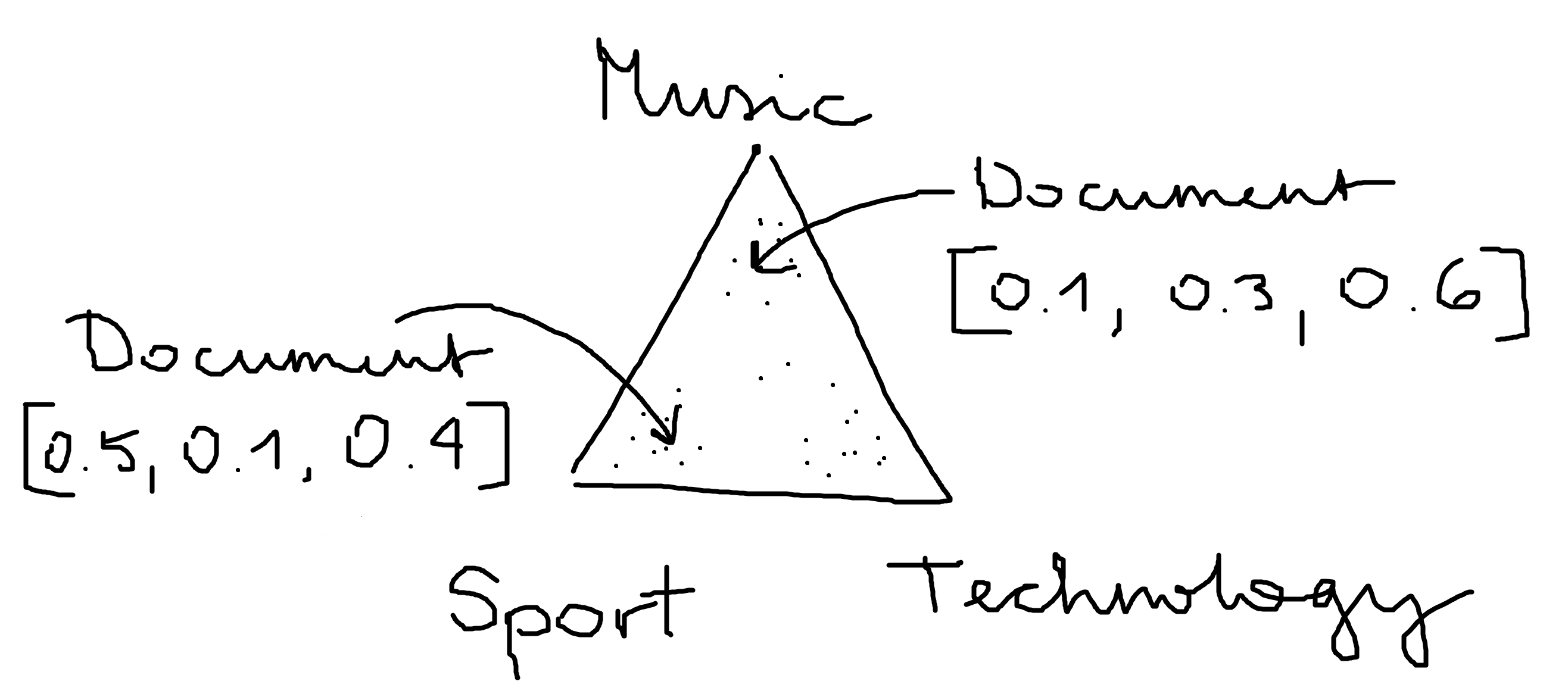
Assume we are given a large collections of documents. Each of these documents can contain text of one or more topics. The goal of a topic model is to infer the topic distribution of each of the documents.
The graph shows a topic model with three topics over a collection of documents.

The latent Dirichlet allocation model
The LDA model is a generative statistical model of a collection of documents. The basic idea is that documents are represented as random mixtures over latent topics, where each topic is characterized by a distribution over words. We describe what we mean by this I a second, first we need to fix some parameters.
- $T$ denotes the number of topics,
- $D$ denotes the number of documents,
- $V$ denotes the number of different works in the vocabulary,
- $N$ is number of words in a given document, so document $i$ has $N_i$ words,
- $w_{ij}$ is the specific $j$-th word in document $i$ and
- $z_{ij}$ is the topic for the $j$-th word in document $i$
Now we can introduce the distribution of topics over the documents, we call it $\theta$. Specifically $\theta_{i}$ is the topic distribution for document $i$, which is just a probability vector. And since each topic is characterized by a distribution over words, we also introduce $\varphi_{k}$ as the word distribution for topic $k.$
Each of our topic distributions of a document is basically a probability vector, so we can view it as a multinomial distribution over the topics. Hence $\theta$ is a distribution over multinomial distributions, which is exactly what a Dirichlet distribution is. The graph we used earlier to represent the mixture of topics in documents re-ensembles the probability density function of a dirichlet distribution with 3 categorical events. So we will model the distribution of topics over the documents $\theta$ and the word distribution for topics $\varphi$ by dirichlet distributions of order $T$, respectively $V$. Other than that we have $\alpha$, the parameter of the Dirichlet prior on the per-document topic distributions and $\beta$, the parameter of the Dirichlet prior on the per-topic word distribution. Usually both parameters are sparse, meaning they are smaller than $1$. We won’t go into the mathematical details of the Dirichlet distributions here and move on the how we can implement the model.
How do we find $\theta$ and $\varphi$? Gibbs sampling!
Now we want to implement the model on real data and discover the latent topics with it. So first we get a text corpus, namely the 20 newsgroup dataset.
import numpy as np
import matplotlib.pyplot as plt
plt.style.use("ggplot")
plt.usetex = True
from tqdm.notebook import tqdm
Get the newsgroup dataset
from sklearn.datasets import fetch_20newsgroups
from sklearn.feature_extraction.text import CountVectorizer
n_samples = 10000
data, _ = fetch_20newsgroups(shuffle=True, random_state=1,
                             remove=('headers', 'footers', 'quotes'),
                             return_X_y=True,
                            )
data_samples = data[:n_samples]
Now we tokenize the text and create a bag of words document representation of our corpus to use in our model.
tf_vectorizer = CountVectorizer(max_df=0.95, min_df=2,
                                max_features=10000,
                                stop_words='english')
tf = tf_vectorizer.fit_transform(data_samples)
vocabulary = tf_vectorizer.vocabulary_
docs = []
for row in tf.toarray():
    present_words = np.where(row != 0)[0].tolist()
    present_words_with_count = []
    for word_idx in present_words:
        for count in range(row[word_idx]):
            present_words_with_count.append(word_idx)
    docs.append(present_words_with_count)
Implement LDA with Gibbs sampling
We first fix some variables as before.
D = len(docs)        # number of documents
V = len(vocabulary)  # size of the vocabulary
T = 10               # number of topics

alpha = 1 / T         # the parameter of the Dirichlet prior on the per-document topic distributions
beta = 1 / T        # the parameter of the Dirichlet prior on the per-topic word distribution
What Gibbs sampling does in its most standard implementation, is it just cycles through all variables and model parameters and randomly samples each one from a conditional distribution where we’re conditioning on the previously sampled values of all the other model parameters and assignment variables, and we’re also conditioning on our observations. Because of the special structure of our LDA model, we can actually analytically marginalize over all of the uncertainty in our model parameters and just sample the word assignment variables $z_{ij}$. This is called “collapsed gibbs sampling”.
We do the sampling of a new topic $z_{ij}$ for a word $w_{ij}$ by the following formula $$P(z_{ij} | z_{kl}\ \text{with}\ k\neq i\ \text{and}\ l \neq j, w) = \frac{\theta_{ik} + \alpha}{N_i + \alpha T} \frac{\phi_{kw} + \beta}{\sum_{w\in V} \phi_{kw} + \beta V}$$
z_d_n = [[0 for _ in range(len(d))] for d in docs]  # z_i_j
theta_d_z = np.zeros((D, T))
phi_z_w = np.zeros((T, V))
n_d = np.zeros((D))
n_z = np.zeros((T))

## Initialize the parameters
# m: doc id
for d, doc in enumerate(docs):
    # n: id of word inside document, w: id of the word globally
    for n, w in enumerate(doc):
        # assign a topic randomly to words
        z_d_n[d][n] = n % T
        # get the topic for word n in document m
        z = z_d_n[d][n]
        # keep track of our counts
        theta_d_z[d][z] += 1
        phi_z_w[z, w] += 1
        n_z[z] += 1
        n_d[d] += 1

for iteration in tqdm(range(10)):
    for d, doc in enumerate(docs):
        for n, w in enumerate(doc):
            # get the topic for word n in document m
            z = z_d_n[d][n]

            # decrement counts for word w with associated topic z
            theta_d_z[d][z] -= 1
            phi_z_w[z, w] -= 1
            n_z[z] -= 1

            # sample new topic from a multinomial according to our formula
            p_d_t = (theta_d_z[d] + alpha) / (n_d[d] - 1 + T * alpha)
            p_t_w = (phi_z_w[:, w] + beta) / (n_z + V * beta)
            p_z = p_d_t * p_t_w
            p_z /= np.sum(p_z)
            new_z = np.random.multinomial(1, p_z).argmax()

            # set z as the new topic and increment counts
            z_d_n[d][n] = new_z
            theta_d_z[d][new_z] += 1
            phi_z_w[new_z, w] += 1
            n_z[new_z] += 1
What to do with the model
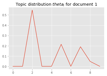
After fitting the model we get the topic distribution over every document encoded in $\theta$
i = 1
plt.plot(theta_d_z[i]/ sum(theta_d_z[i]));
plt.title("Topic distribution $theta_i$ for document {}".format(i));

For example we can look at the most probable words per topic by looking at the distribution over words for topic $k$ in $\varphi_k$.
inv_vocabulary = {v: k for k, v in vocabulary.items()}
n_top_words = 10
for topic_idx, topic in enumerate(phi_z_w):
    message = "Topic #%d: " % topic_idx
    message += " ".join([inv_vocabulary[i] for i in topic.argsort()[:-n_top_words - 1:-1]])
    print(message)
Topic #0: 00 10 20 25 15 12 team 11 game 16
Topic #1: edu file com mail available information ftp use image thanks
Topic #2: god people think don does mr believe law know just
Topic #3: just like don know time car good problem does think
Topic #4: people just don like know think said right time did
Topic #5: key use space encryption chip used new information technology law
Topic #6: use drive windows scsi does using card bit like disk
Topic #7: said people don think going know like just let ll
Topic #8: people government armenian turkish war jews public world new armenians
Topic #9: ax max g9v db pl b8f a86 cx 75u 145
This looks very reasonable. I hope this article helped you gain as much understanding about LDA as it did for me (which was quite a lot!). You can find out more about the application of this model in another blog post of mine.
Resources
