Since a lot of people recently asked me how neural networks learn the embeddings for categorical variables, for example words, I’m going to write about it today. You all might have heard about methods like word2vec for creating dense vector representation of words in an unsupervised way. With this words you would initialize the first layer of a neural net for arbitrary NLP tasks and maybe fine-tune them. But the use of embeddings goes far beyond that! We can use them to learn supervised representations of arbitrary categorical variables. This makes embeddings a powerful tool for handling categorical data.
But how does this work and what is the idea behind it? After reading this article, you will know:
- What an embedding layer really is.
- How neural nets can learn representations for categorical variables.
- How fine-tuning of word vectors works.
What is an embedding layer?
Our setup is the following:
- we got a categorical variable with multiple categories as input for our network. This can be words, size of shoes or weather conditions. Note, that the number of categories can be easily in the hundreds of thousands.
- We have a target variable that we want to learn the representation of our categories from.
To understand how it works we first do the math. We start with a vector (our categorical variable) $X$, that looks like this
$$ X=(0,1,2,2). $$
Every entry in $X$ represents a different sample. We also got a target vector $y$ which represents a binary random variable we try to predict.
$$ y = (1,1,0,0)^T. $$
We represent $X$ by one-hot encoding the categories, where each dimension stands for one possible category, e.g. a word in our vocabulary. Then it looks like this in numpy:
import numpy as np

X = np.array([
    [1,0,0],  # Category 1
    [0,1,0],  # Category 2
    [0,0,1],  # Category 3
    [0,0,1]   # Category 3
])

y = np.array([[1,1,0,0]]).T
We set up $y$ such that the categories one and two have positive label and category three has negative label. So we can reason about the toy task later. We use a simple neural network architecture with one hidden layer like this.
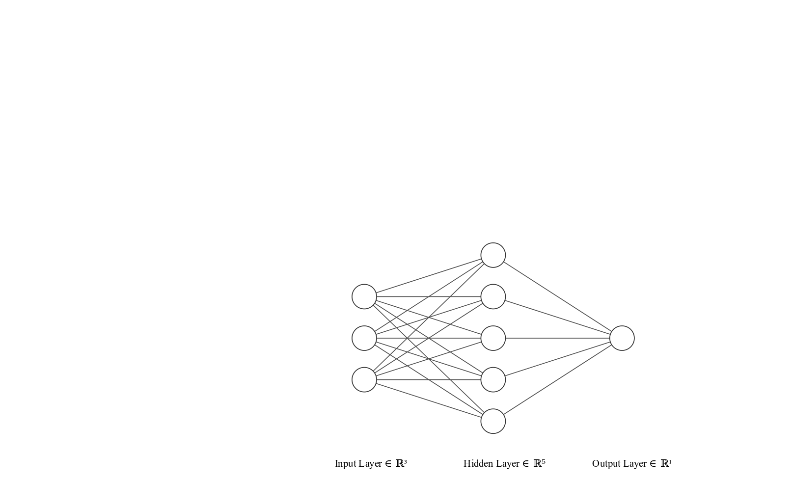
The math
The lines connecting the nodes are the weights or parameters of the neural network. In our case they are matrices of dimensions $(3, 5)$ and $(5, 1)$. We write them as $W_0$ and $W_1$, respectively. We get from one layer to the next by multiplying the output of the previous layer by the respective weights. The first layer is the input layer, which is basically just our input data $X$. As we discussed, every row in the matrix $X$ is a vector with exactly one $1$ and all other values $0$. The $1$ stands for the category value for the sample.
So what happens if we multiply the vector of our first sample $X_1 = (1,0,0)$ by the weights $W_0$?
$$ (1,0,0) * W_0 = (w_{00}, w_{01}, w_{02}, w_{03}, w_{04})^T,$$
which is the first row of the weight matrix. This is what we call the embedding matrix. We use only a linear activation afterwards and put the embedding directly to the next layer. So the embedding layer is basically a linear neural network layer that can be updated with backpropagation.
Build a simple embedding network
We now build the above architecture in python and numpy. Then we train the embeddings with backpropagation and investigate the embeddings.
To understand what the code does you should read the excellent tutorial (where the basic code is from) here: https://iamtrask.github.io/2015/07/12/basic-python-network/
n_categories = 3  # number of possible categories
emb_dim = 5       # dimension of the emdedding vectors
# initialize the weights
weights0 = 2*np.random.random((n_categories, emb_dim)) - 1
weights1 = 2*np.random.random((emb_dim, 1)) - 1
def sigmoid(x, deriv=False):
    if(deriv == True):
        return x * (1 - x)
    return 1 / (1 + np.exp(-x))
learning_rate = 0.1


for j in range(60000):
    # forward pass
    output1 = np.dot(X, weights0)  # A linear hidden layer
    output2 = sigmoid(np.dot(output1, weights1))  # Output layer with sigmoid activation
    # computing error
    l2_error = y - output2
    if (j% 10000) == 0:
        print("Error:" + str(np.mean(np.abs(l2_error))))
    # backward pass
    l2_delta = l2_error * sigmoid(output2, deriv=True)
    l1_error = l2_delta.dot(weights1.T)
    l1_delta = l1_error
    # update the weigths
    weights1 += learning_rate * output1.T.dot(l2_delta)
    weights0 += learning_rate * X.T.dot(l1_delta)
Error:0.5646094252817514
Error:0.004711527936056814
Error:0.0031925862947534966
Error:0.0025482109342667442
Error:0.0021733418432724944
Error:0.0019217982856947961
output2
array([[0.99805614],
       [0.99795945],
       [0.00148479],
       [0.00148479]])
We can see the error going down quickly in our toy task and the prediction is correct.
Investigate the embeddings
Now we investigate the hidden layer of this network.
weights0
array([[ 0.63279519,  1.18772108,  0.62115838, -0.82322761, -1.56834962],
       [ 0.47705258, -0.1903559 ,  1.61830164, -0.04156358, -1.52883417],
       [ 1.03534223, -1.29040755, -1.14544297,  0.27858696,  0.85634903]])
Every row in this matrix is our embedding for the respective category now. Now we compare the embeddings for the different categories by cosine similarity.
from scipy import spatial
spatial.distance.cosine(weights0[0], weights0[1])
0.3343839640045886
spatial.distance.cosine(weights0[0], weights0[2])
1.620888998379765
spatial.distance.cosine(weights0[1], weights0[2])
1.4833413128320145
So we see, that the network learned some useful representation for the categories in our toy task. The first and the second category are quite close, while both of them are far away from the third category. If you remember the setup of the task, this totally makes sense.
Do it with keras
Now we move the architecture and the setup to keras and see how it works.
from keras.models import Sequential
from keras.layers import Embedding, Flatten, Dense, Activation
from keras.optimizers import SGD
model = Sequential()
model.add(Embedding(input_dim=n_categories, output_dim=emb_dim, input_shape=(1,)))
model.add(Flatten())
model.add(Dense(units=1, activation="sigmoid"))
sgd = SGD(lr=learning_rate)
model.compile(optimizer=sgd, loss="binary_crossentropy", metrics=["accuracy"])
Note, that keras handles the one-hot encoding internally, so you have to pass integer indices for your categories. This is why we used argmax to get the category index.
model.fit(np.argmax(X, axis=1), y, epochs=5);
Epoch 1/5
4/4 [==============================] - 0s 44ms/step - loss: 0.7012 - acc: 0.5000
Epoch 2/5
4/4 [==============================] - 0s 633us/step - loss: 0.6838 - acc: 0.5000
Epoch 3/5
4/4 [==============================] - 0s 300us/step - loss: 0.6670 - acc: 1.0000
Epoch 4/5
4/4 [==============================] - 0s 507us/step - loss: 0.6509 - acc: 1.0000
Epoch 5/5
4/4 [==============================] - 0s 3ms/step - loss: 0.6352 - acc: 1.0000
keras_embs = model.layers[0].get_weights()[0]
keras_embs
array([[ 0.02557688,  0.03779284, -0.05189876,  0.06510007, -0.03094837],
       [ 0.00011533,  0.05283174, -0.05359174,  0.03876735, -0.06703786],
       [-0.00463526, -0.0850474 ,  0.07373089, -0.02540122,  0.07149601]],
      dtype=float32)
spatial.distance.cosine(keras_embs[0], keras_embs[1])
0.1301671862602234
spatial.distance.cosine(keras_embs[0], keras_embs[2])
1.8129135370254517
spatial.distance.cosine(keras_embs[1], keras_embs[2])
1.9697489142417908
So the results on the toy task agree quite well between our numpy implementation and the keras implementation. So now that you understood embeddings, you can go on and try them with keras in a non-toy task.