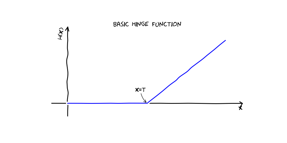
In this post we will introduce multivariate adaptive regression splines model (MARS) using python. This is a regression model that can be seen as a non-parametric extension of the standard linear model.
The multivariate adaptive regression splines model
MARS builds a model of the from
$$f(x) = \sum_{i=0}^k c_i B_i(x_i),$$
where $x$ is a sample vector, $B_i$ is a function from a set of basis functions (later called terms) and $c_i$ the associated coefficient.
The basis functions are one of the following:
- constant 1, the so called intercept to reduce bias,
- a hinge function $h(x) = \max(0, x – t)$ or $\max(0, t - x)$ (also called rectifier functions), where $t$ is a constant, to model non-linearities,
- a product of two or more hinge functions to automatically model interactions between features.

How do we learn?
The MARS algorithm does learning in two steps. First we overgenerate a set of basis functions in the so called “forward pass”. The forward pass searches for terms that locally minimize squared error loss on the training set. Here we just add basis functions in a greedy way one after another. In The second step, the “pruning pass”, we remove unnecessary basis functions. The pruning pass uses generalized cross validation (GCV) to compare the performance of model subsets in order to choose the best subset: lower values of GCV are better. The GCV is a form of regularization: it trades off goodness-of-fit against model complexity.
The formula for the GCV is $$GCV = \frac{RSS}{(N (1 - EffectiveNumberOfParameters / N)^2)}$$ where RSS is the residual sum-of-squares measured on the training data and N is the number of trainingsamples.
The EffectiveNumberOfParameters is defined in the MARS context as $$EffectiveNumberOfParameters = n_{terms} + penalty \frac{(n_{terms} - 1 )}{2}.$$ The GCV formula penalizes the addition of terms. Thus the formula adjusts the training RSS to take into account the flexibility of the model. We penalize flexibility because models that are too flexible will model the specific realization of noise in the data instead of just the systematic structure of the data.
A working example in python
Now we will look at a working example in python. For this we use the implementation provided by the pyearth package. We will use the data set from the “House Prices: Advanced Regression Techniques” challenge on kaggle. The data set contains 79 explanatory variables describing (almost) every aspect of residential homes in Ames, Iowa, this competition challenges you to predict the final price of each home.
import pandas as pd

import numpy as np
from scipy.stats import skew
from scipy.stats.stats import pearsonr

train = pd.read_csv("data/train.csv")
test = pd.read_csv("data/test.csv")

all_data = pd.concat((train.loc[:,'MSSubClass':'SaleCondition'],
                      test.loc[:,'MSSubClass':'SaleCondition']))
We start with some basic data processing. We’re not going to do anything fancy here:
- First I'll transform the skewed numeric features by taking $\log(feature + 1)$, this will make the features more normal
- Create Dummy variables for the categorical features
- Replace the numeric missing values (NaN's) with the mean of their respective columns
#log transform the target:
y = np.log1p(train["SalePrice"])

#log transform skewed numeric features:
numeric_feats = all_data.dtypes[all_data.dtypes != "object"].index

skewed_feats = train[numeric_feats].apply(lambda x: skew(x.dropna())) #compute skewness
skewed_feats = skewed_feats[skewed_feats > 0.75]
skewed_feats = skewed_feats.index

all_data[skewed_feats] = np.log1p(all_data[skewed_feats])
X_train = all_data[:train.shape[0]]
X_test = all_data[train.shape[0]:]
About model parameters
The pyearth MARS model offers some parameters to tune. I list the most important ones and how they influence the model.
- max_terms: The maximum number of terms generated by the forward pass. Decreasing the number will reduce overfitting but can also limit the expressiveness of the model. Typically only one or two degrees of interaction are allowed, but higher degrees can be used when appropriate.
- max_degree: The maximum degree of terms generated by the forward pass. Increasing this parameter will increase the non-linearity of the model but can lead to overfitting and increase the computation time a lot.
- penalty: The penalty parameter used to calculate GCV. Used during the pruning pass and to determine whether to add a hinge or linear basis function during the forward pass.
from sklearn.model_selection import cross_val_score
from pyearth import Earth

def rmse_cv(model):
    rmse= np.sqrt(-cross_val_score(model, X_train, y, scoring="neg_mean_squared_error", cv = 5))
    return(rmse)

mars = Earth(max_degree=1, penalty=1.0, endspan=5)

cv_mars = rmse_cv(mars).mean()

print(cv_mars)
This gives us a rooted mean squared logarithmic error of 0.126. Looks not so bad. This is definitely a good start.
Go further with boosted MARS
We can use the MARS model like decision trees for boosting. Scikit-learn offers a convenient way to do this with the AdaBoostRegressor. Just plug it in there and here we go:
from sklearn.ensemble import AdaBoostRegressor

boosted_model = AdaBoostRegressor(base_estimator=mars, n_estimators=25,
                                  learning_rate=0.1, loss="exponential")
All this features make the MARS model a very handy tool in your machine learning toolbox.
Go out and use it!
